Exploring diabetes indicators across the US
First Post
This material is from a learning project. I wanted to learn some rmarkdown and how to work with the sf package and ggplot2’s geom_sf(). It is not a polished write up (or analysis) but it’s a good first post to help me set up a workflow for posting to this site. All the R code can be found on GitHub.
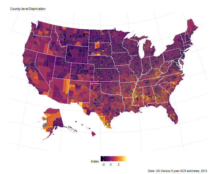
County level deprivation index
Details about the index can be found here. In short, estimates are collected from the American Community Survey and a principal component analysis extracts a deprivation score for each observation. Higher index scores represent higher area deprivation relative to all other counties in the US.
For this project, the index was calculated using 5-year ACS estimates from 2013, at the county-level, to link to the available diabetes dataset.
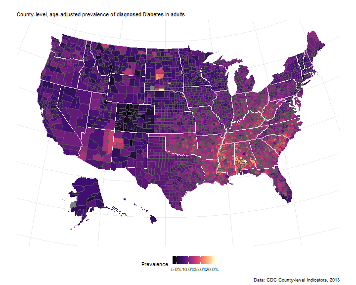
Diabetes Indicators
National data on diabetes indciators are available from the CDC. Indicator estimates are the most up to date as of 2013 and available at the county-level only. Indicators (age-adjusted) are: 1. prevalence of diagnosed diabetes, 2. prevalence of obesity, and 3. prevalence of leisure-time physical inactivity, hereafter just inactivity.
The spatial distribution of diabetes prevalence in 2013 (below) parallels that of 2007, which led to the recognition of a “diabetes belt” in the southern United States.
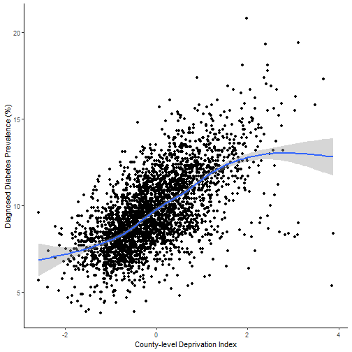
Data Analysis
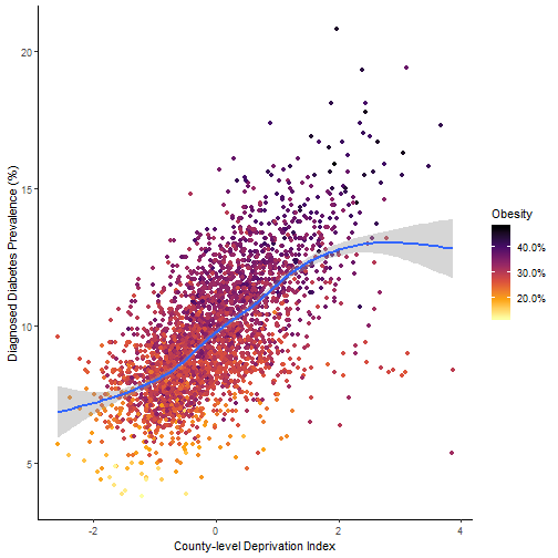
Obesity and physical inactivity are well-known risk factors for developing diabetes. Therefore, in order to assess whether area deprivation is associated with diabetes prevalence, independent of obesity and inactivity, a blocked multiple regression was fitted. First we estimated the effects of obesity and inactivity; then, the deprivation variable was introduced.
Regression results
library(stargazer, quietly = TRUE)

stargazer(lm1,lm2, type ="html")
| Dependent variable: | ||
| DiabPrev | ||
| (1) | (2) | |
| ObPrev | 0.188*** | 0.165*** |
| (0.008) | (0.007) | |
| InactPrev | 0.192*** | 0.132*** |
| (0.007) | (0.007) | |
| PC1 | 0.740*** | |
| (0.031) | ||
| Constant | -0.912*** | 1.311*** |
| (0.166) | (0.180) | |
| Observations | 3,142 | 3,142 |
| R2 | 0.601 | 0.661 |
| Adjusted R2 | 0.600 | 0.660 |
| Residual Std. Error | 1.383 (df = 3139) | 1.275 (df = 3138) |
| F Statistic | 2,361.260*** (df = 2; 3139) | 2,035.008*** (df = 3; 3138) |
| Note: | *p<0.1; **p<0.05; ***p<0.01 | |
Increases in county-level deprivation predict increases in diabetes prevalence.
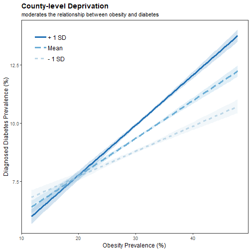
Interaction Term
Results summary
## MODEL INFO:
## Observations: 3142 (79 missing obs. deleted)
## Dependent Variable: DiabPrev
## Type: OLS linear regression
##
## MODEL FIT:
## F(4,3137) = 1668.00, p = 0.00
## R² = 0.68
## Adj. R² = 0.68
##
## Standard errors: OLS
##             Est. S.E. t val.    p
## (Intercept) 9.50 0.02 400.02 0.00 ***
## InactPrev   0.14 0.01  19.71 0.00 ***
## ObPrev      0.16 0.01  22.99 0.00 ***
## PC1         0.68 0.03  22.08 0.00 ***
## ObPrev:PC1  0.06 0.00  13.90 0.00 ***
##
## Continuous predictors are mean-centered.
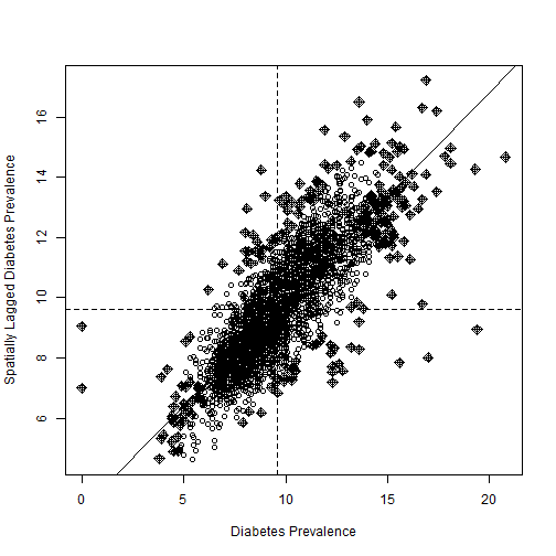
Spatial Auto-correlation of county prevalence
##
## 	Moran I test under randomisation
##
## data:  MapSP$diabetes
## weights: nb2listw(neighbors)
## omitted: 1543, 3118
##
## Moran I statistic standard deviate = 67.205, p-value < 2.2e-16
## alternative hypothesis: greater
## sample estimates:
## Moran I statistic       Expectation          Variance
##      0.6962110037     -0.0003185728      0.0001074177
MapSP$diabetes <- ifelse(is.na(MapSP$diabetes), 0, MapSP$diabetes)
moran.plot(MapSP$diabetes,nb2listw(neighbors), zero.policy = FALSE,
           labels = FALSE,main=c(" "),
           xlab="Diabetes Prevalence",ylab = "Spatially Lagged Diabetes Prevalence")